Sun Exposure, Skin Cancer, and a Methodological Sunburn

In 2013, Brøndum-Jacobsen and colleagues published a study in the International Journal of Epidemiology testing whether sun exposure (proxied by skin cancer diagnosis) was associated with better downstream health outcomes. The logic is biologically plausible: more sun means more vitamin D, with downstream effects on bone metabolism and cardiovascular function.

The dataset is exceptional. The investigators used linked Danish national registries covering the entire Danish population above age 40 from 1980 to 2006: 4.4 million individuals. Denmark's administrative registers are among the most valuable resources in epidemiology: every resident carries a unique civil registration number (CPR) assigned at birth, enabling exact linkage across the National Patient Registry, the Cancer Registry, the Civil Registration System, and the Cause of Death Registry. No sampling, no recall bias, near-complete ascertainment of diagnoses and deaths across a quarter century.

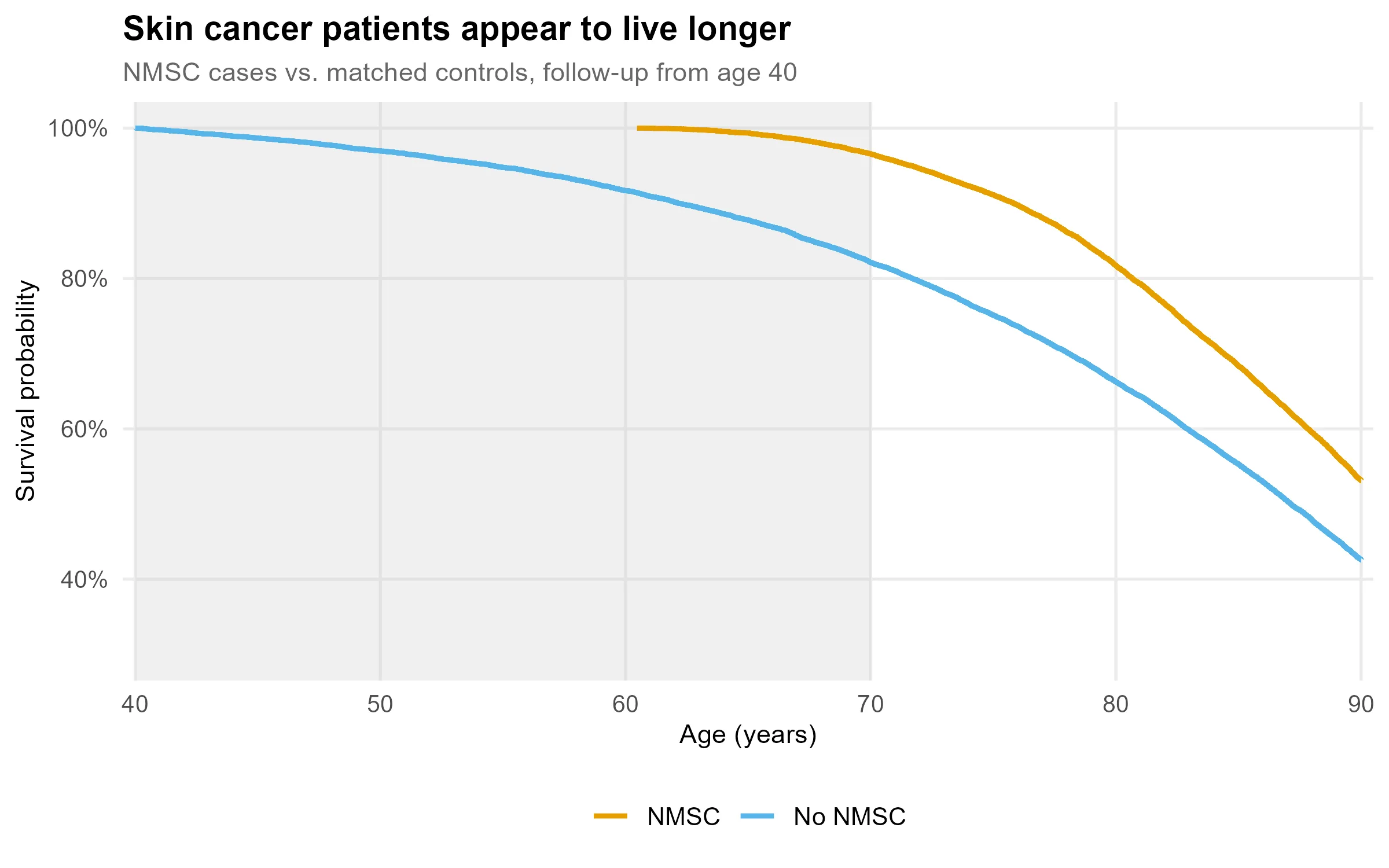
The results were striking. Compared to the general population:

• Patients with non-melanoma skin cancer (NMSC) had an adjusted HR = 0.52 for all-cause mortality: risk of dying apparently halved.
• They also had lower rates of myocardial infarction and, in those under 90, lower rates of hip fracture.
• Melanoma patients showed a similar but attenuated pattern: HR = 0.89 for all-cause mortality.

The mechanisms seem to write themselves: sun exposure, vitamin D synthesis, calcium metabolism, stronger bones, fewer fractures. Or nitric oxide, vasodilation, lower cardiovascular mortality. Both pathways are real. The confidence intervals are razor-thin from the enormous sample size, and the consistency across outcomes is persuasive. The authors were careful: "Causal conclusions cannot be made from our data." But effect sizes like these rarely stay confined to their caveats.

The simulation below reproduces the study design under the assumption that skin cancer has zero causal effect on mortality. Mortality is drawn from a Gompertz model calibrated to Danish population life tables. The grey band marks the immortal time window.

The Problem

NMSC (basal cell carcinoma and squamous cell carcinoma) accumulates over a lifetime of sun exposure and is typically diagnosed between ages 60 and 80, well after the study's age-40 entry point.

To appear in the NMSC group, a patient had to survive to their diagnosis date. A person diagnosed at age 72 was, by definition, alive from age 40 to 72. That 32-year window is immortal time: they could not have died during it and still received a diagnosis. Yet this entire span enters the analysis as person-time, compared against a general population that includes everyone who died at 45, 55, or 65, before any diagnosis was possible.

The exposed group accrues a guaranteed survival advantage that has nothing to do with sun exposure, vitamin D, or any biological mechanism.

To isolate this, consider a thought experiment: instead of a skin cancer diagnosis, we award a lottery prize to a random subset of the cohort at a random age between 70 and 80. No selection on health. No biology. We then run the same analysis, comparing prize winners to non-winners for all-cause mortality from age 40.

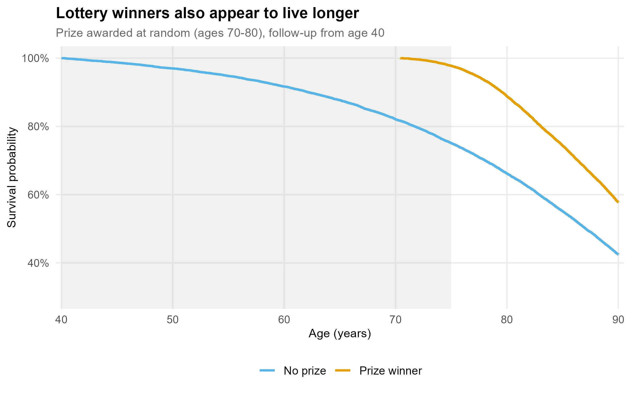
The prize produces a larger apparent protective effect than the skin cancer diagnosis. This is purely because it is awarded later. The magnitude of immortal time bias scales directly with how late the qualifying event occurs, which is also why the NMSC effect (HR = 0.52, diagnosed in the 60s–80s) dwarfs the melanoma effect (HR = 0.89, diagnosed earlier and itself directly lethal). The biology is beside the point; the timing explains the result.

The Correction

Rather than starting follow-up at age 40 for everyone, we start at the prize award date. Controls are assigned a pseudo-prize at the same age as their matched case. Both groups now begin observation at the same point; the immortal window is removed.

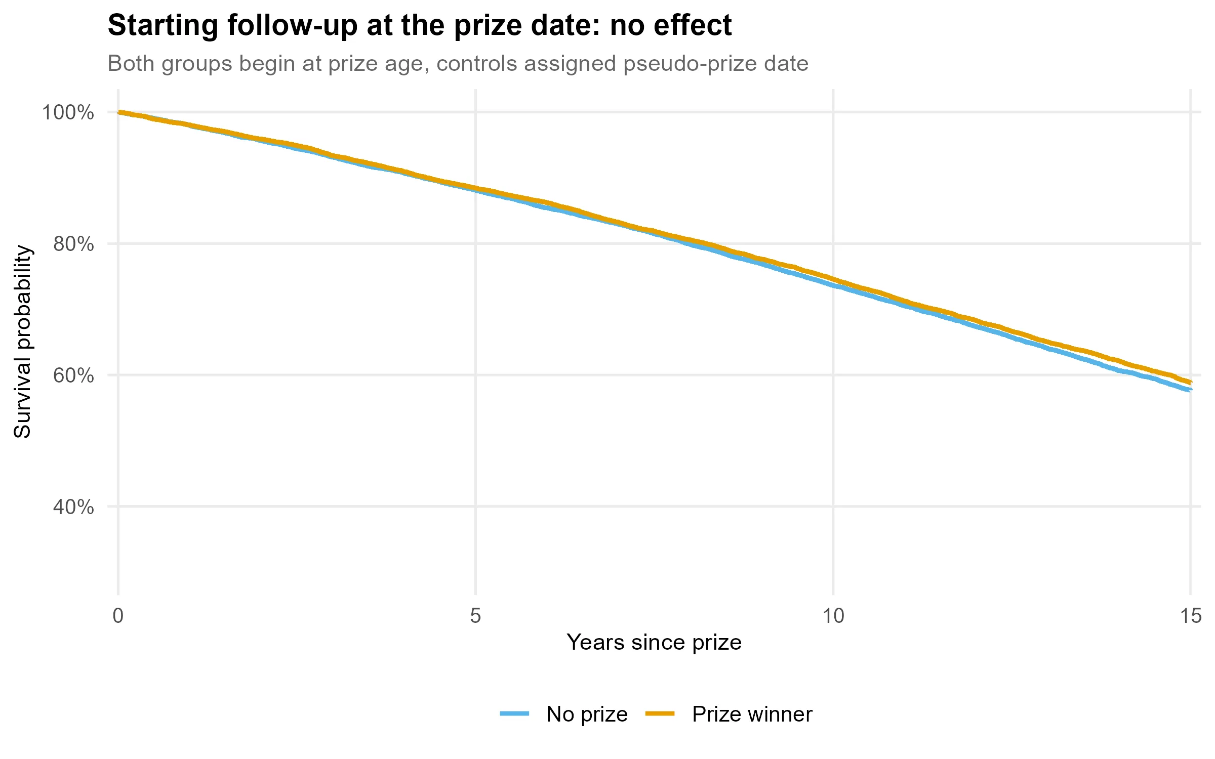
The equivalent correction in the original study would be to use the skin cancer diagnosis date as the index date, counting only person-time after diagnosis, or to model exposure as a time-varying covariate in a Cox model, where each individual contributes unexposed time until diagnosis and exposed time thereafter.

Take-Home

Immortal time bias is structurally invisible in the most common study designs: large registry cohorts, long follow-up, exposures defined by events that require surviving to experience them. These are also the conditions associated with high-powered, high-credibility studies. The bias does not appear in any coefficient; it lives in the denominator.

The lottery exercise makes the diagnostic explicit. If replacing the exposure with something biologically inert produces the same result, the exposure is not doing the work.

In matched or registry-based cohort studies, the key question is simple: does follow-up start at the same calendar time for cases and controls? If cases are defined by a post-baseline event and controls are not subject to that constraint, you are likely looking at immortal time.

library(survival)
set.seed(42)

# Gompertz mortality: h(t) = a*exp(b*t), t = years since age 40
# Calibrated to Danish adult life tables (~age 87 median survival)
sim_death_age <- function(n, a = 0.00195, b = 0.0685) {
  u <- runif(n)
  40 + (1/b) * log(1 - (b/a) * log(1 - u))
}

n <- 20000
death_case    <- sim_death_age(n)
death_control <- sim_death_age(n)
obs_case    <- pmin(death_case, 90)
obs_control <- pmin(death_control, 90)

# Prize awarded at random (ages 70-80); no biological mechanism
prize_age <- runif(n, 70, 80)
won <- prize_age <= obs_case

# Biased: follow-up from age 40
biased <- data.frame(
  time  = c(obs_case[won] - 40, obs_control[won] - 40),
  event = c(death_case[won] <= 90, death_control[won] <= 90),
  prize = rep(c(1, 0), each = sum(won))
)
coxph(Surv(time, event) ~ prize, data = biased) |> coef() |> exp()
# prize: ~0.57

# Correct: follow-up from prize date, controls assigned matched pseudo-prize
alive <- death_control[won] > prize_age[won]
correct <- data.frame(
  time  = c(obs_case[won][alive] - prize_age[won][alive],
            obs_control[won][alive] - prize_age[won][alive]),
  event = c(death_case[won][alive] <= 90, death_control[won][alive] <= 90),
  prize = rep(c(1, 0), each = sum(alive))
)
coxph(Surv(time, event) ~ prize, data = correct) |> coef() |> exp()
# prize: ~0.97